Methods

• Description of the tools and techniques used to solve the problem stated in the introduction

  • Stream nodes and their corresponding simulated groundwater heads obtained from CV2SIM-FG v1.5

  • A streamline for the Sacramento River was prepared by connecting C2VSIM-FG v1.5 stream nodes. [California Department of Water Resources, 2025].

  • Groundwater table elevations were calculated equal to the simulated groundwater head of the highest layer where the head was above the layer bottom elevation, for each stream node and timestep.

  • Lithology logs were obtained from DWR’s Airborne Electromagnetic Survey (AEM) for survey areas 6 [California Department of Water Resources, 2023] and 7 [California Department of Water Resources, 2023]. Only logs labeled as high quality (HQ) were used.

  • Textures described in the AEM lithology logs were grouped into broader categories to reduce the number of patterns necessary for displaying them in the transects. The grouping was conducted according to the following table:

    Texture	Plotting Group
    Boulders	Gravel
    Clay	Clay
    Cobbles	Gravel
    Gravel	Gravel
    Rock - Intrusive	Rock
    Rock - Metamorphic	Rock
    Rock - Sedimentary	Rock
    Rock - Undifferentiated	Rock
    Rock - Volcanic	Rock
    Sand	Sand
    Silt	Silt
    Soil	Soil
    Unknown	Unknown

  • Measured groundwater levels were obtained from CASGEM [California Department of Water Resources, 2025]

  • CASGEM and lithology wells within 500 m (1,640.42 ft) from the Sacramento River streamline were projected to the streamline and used for the analysis.

  • Observation wells overlap in the transect were solved based on the following criteria:

    • For multicompletion wells, the shallowest piezometer was selected. If the shallowest piezometer was too shallow (less than 20 ft) the next one in depth order was chosen.

    • Observation wells were prefered over irrigation and domestic wells

    • Shallow wells were preferred over deep wells.

    • Where all the overlapping wells were shallow observation wells, the projected distance into the transect was manually adjusted to make the labels for both wells visible

  • Bathymetry was sampled at C2VSIM-FG v1.5 stream nodes along the Sacramento River from [Yurok Tribe and US Bureau of Reclamation, 2024] and [Wang et al., 2019].

  • We selected 190 mi between Sacramento and Red Bluff for our analysis. This section was divided into three transects for ease of plotting. Transect distances are reported in miles upstream from the confluence between the Sacramento River and the San Joaquin River.

    • The southern transect spans from miles 50 to 120, approximately corresponding to the latitudes of Sacramento and Yuba City.

    • The central transect spans from miles 120 to 190, approximately corresponding to the latitudes of the Yuba City and Chico boundary.

    • The northern transect spans from miles 190 to 240, approximately corresponding to the latitudes of Chico and Red Bluff.

  • The data processing was carried out in Python using libraries rasterio [Gillies and others, 2013], shapely [Gillies et al., 2025], pandas [McKinney, 2010], geopandas [Jordahl et al., 2020], and numpy [Harris et al., 2020]. Animated transects and maps were plotted using matplotlib [Hunter, 2007]. Deployment was handled using jupyter book [Executable Books Community, 2020] and GitHub Pages [GitHub, n.d.].

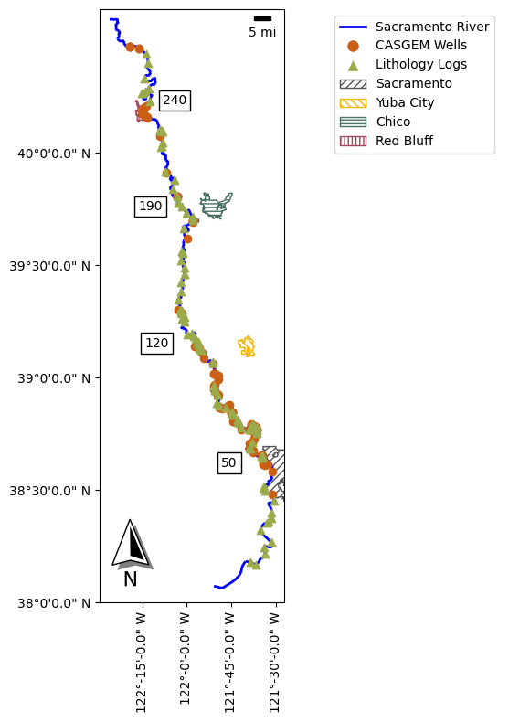
Fig. 1 Sacramento River and selected CASGEM wells and lithology logs. Distance along the Sacramento River from the confluence with the San Joaquin River at transect sections boundaries are shown in white boxes in units of miles.